If you are an analyst, regardless of your job sector, you are aware that there are many different approaches to stock market prediction. The most relevant ones today mostly use neural networks applied to sequence data, such as LSTMs, or involve sentiment analysis and signal detection.

These approaches are interesting, and for a good reason — there are plenty of resources on the internet that deals with the topics mentioned. That’s not a bad thing, as analysts can initiate their projects following a shared baseline and then expand with their methodologies.

Today I want to propose a different approach, one that I dreamt about a couple of weeks ago and that kept me thinking because of the unexpected opportunities. I am talking about time series clustering applied to stock markets.

My main thought was

What if I could identify patterns in data, find similar patterns, group them and assign investment opportunities to each pattern?

This would allow me to spot relevant sequences that could predict a specific trend in a probabilistic fashion.

I have put some hours into this project, and I would like to share with you the first part of this series. As I keep on working on this project, I will share my findings in another article.

Keep in mind that this is my approach — if you like the overall reasoning, but you’d do something different, please let me know with a comment 👌

I hope you are excited as I am about this project. Let’s get started!

The underlying intuition

The idea is that if we take a time series, regardless of its nature and context (be it a stock or anything else), we can divide it into chunks and study each chunk in isolation.

This allows us to make hypotheses on these chunks and to test one against another.

Speaking of which — this is the hypothesis for this problem

If I divide a time series into chunks of a specific length, I can then split the chunks into two parts, which I'll call A and B. B will therefore always follow A.

By studying A, I can find patterns and group elements that behave similarly. This allows me to compute the probability that B following certain A share a similar trend.

The probabilistic approach seems to me to be the most suited one. You'll see why in just a bit.

Bottom line, I want to find portions of a trend that occur with a certain degree of similarity in the whole time series. I want to group these similar portions and see how the portion that follows behaves in terms of trend, which is computed using the slope.

Here's a diagram of how I imagined solving this problem

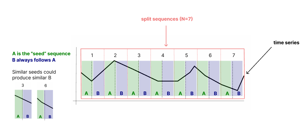
If we find that some As share a high degree of similarity, then we can group them together and find the probability of B going up or down by counting how many Bs have a positive or negative slope.

The algorithm

Given the explanation above, here's how I have designed the algorithm

1. Split the time series into sequences of length N

2. Split each sequence into two parts based on size K to create A and B sequences.

3. Compute the similarity S among all sequences of A

4. Group all similar sequences of A based on a threshold

5. For each group G, compute the probability P of a positive, negative, o stable trend in the sequence B

6. In a new, unseen time series, identify the grouped sequence A to get the probability of the following portion B

If these steps aren't perfectly clear for you at the moment, worry not. I'll explain each step with detailed argumentation and with code.

Let's start right away with coding this.

Requirements

We are going to code the logic from scratch, so we’ll just rely on a handful of Python libraries.

# data manipulation
import pandas as pd 
import numpy as np

# viz
import matplotlib.pyplot as plt
import seaborn as sns

# time and date libs
import datetime

# stock data access
import pandas_datareader as pdr

The only mention worth doing here is that we are going to use pandas_datareader as the provider of stock market data. We'll test portions of this algorithm on several tickers.

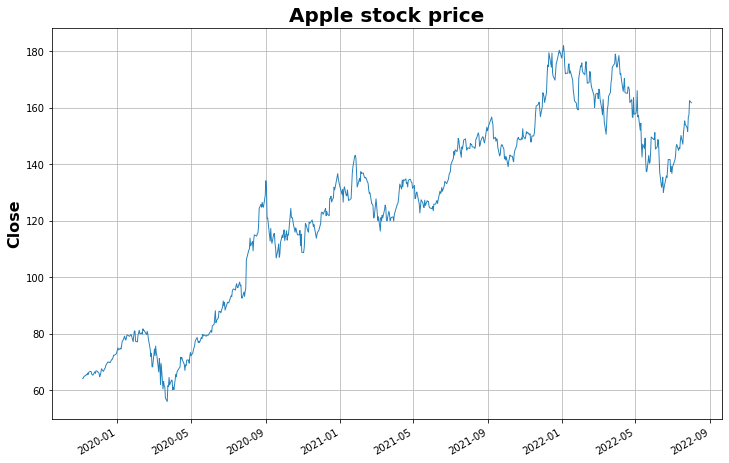
The time series

We are going to use pandas_datareader to pull in stock data on Apple of 1000 days ago. This will include 689 data points. This is because weekends and other holidays are excluded.

There's no particular reason why I chose this number, it just seemed like enough data. Let's define a helper function to do just this.

def get_data(ticker: str, start_date: datetime, end_date: datetime) -> pd.DataFrame:
    """
    Get stock data input ticker
    """
    data = pdr.get_data_yahoo(ticker, start=start_date, end=end_date)
    return data

# get 1000 days of data for Apple starting from today
start_date = datetime.datetime.now() - datetime.timedelta(days=1000)
end_date = datetime.datetime.now()

data = get_data('AAPL', start_date=start_date, end_date=end_date)

data.head()

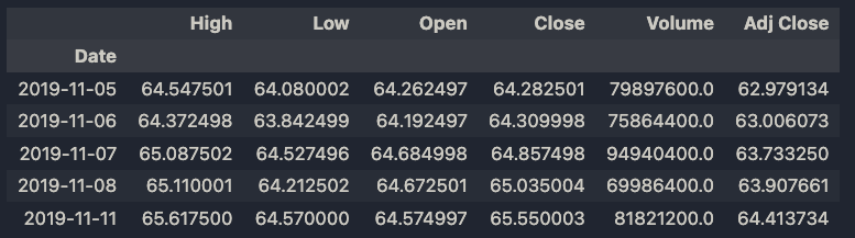
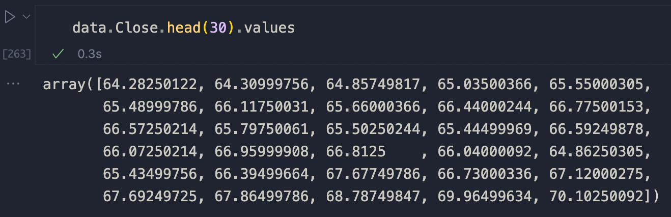
We are going to use the close column as our time series.

Now let's proceed with splitting the time series according to the logic mentioned above.

Split the time series

We are going to define two functions that will split the time series first into sequences and then into split sequences. Let me show you an example:

Suppose we have a Numpy array of 20 numbers

s = np.array([i for i in range(30)])

We want to take this series and split it into N segments of equal size. We can achieve this like so

def split_time_series(series, n):
    """
    Split a time series into n segments of equal size
    """
    split_series = [series[i:i+n] for i in range(0, len(series), n)]
    # if the last sequence is smaller than n, we discard it
    if len(split_series[-1]) < n:
        split_series = split_series[:-1]
    return np.array(split_series)

If we apply this function to s with n = 6 we obtain a complete split sequence with no discarded elements (because there's no remainder when dividing 30 by 6).

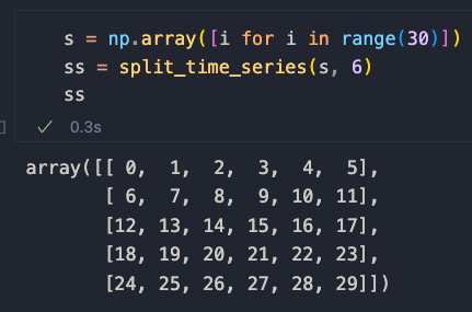
Application of the split_sequence method. Image by the author.

Now we need to split each sequence into two parts based on size K to create A and B sequences. Let's define two new functions called split_sequence and split_sequences for this.

def split_sequence(sequence, k):
    """
    Split a sequence in two, where k is the size of the first sequence
    """
    return np.array(sequence[:int(len(sequence) * k)]), np.array(sequence[int(len(sequence) * k):])


def split_sequences(sequences, k=0.80):
    """
    Applies split_sequence on all elements of a list or array
    """
    return [split_sequence(sequence, k) for sequence in sequences]

In split_sequence, the parameter K allows us how to control the size of the first sequence. See it as the test_size parameter in Sklearn's train_test_split.

split_sequences instead is just responsible for applying the logic to an array.

Let's apply it to our example to understand how it works

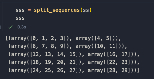
The A and B sequences are defined as so

[seq[0] for seq in sss], [seq[1] for seq in sss]

so the paired elements from the first and second list in the Numpy array.

Let's apply all of this to our time series.

N = 15  # window size --> we can tweak it and test different options
K = 0.70 # split size --> 80% of the data is in A, 20% in B

SEQS = split_time_series(list(data['Close'].values), N) # creates sequences of length N

SPLIT_SEQS = split_sequences(SEQS, K) # splits sequences into individual sequences

A = [seq[0] for seq in SPLIT_SEQS]
B = [seq[1] for seq in SPLIT_SEQS]

If we take a look at A[0] and B[0] we get the first portion of Apple's close data, showing that the preprocessing was successful.

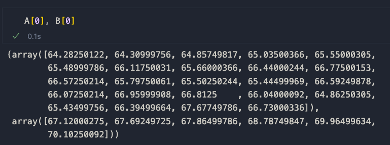
Now we are ready to compare sequences through similarity.

Similarity computation

This is the third step of the algorithm. In order to compute similarity, we’ll use a combination of Pearson’s correlation and dynamic time warping. The correlation helps us match the general direction of the trends, while DTW helps us compute the distance between points. There are plenty of resources online on these two topics, and I suggest you check them out if you are interested.

The formula is the following, and it is a weighted product of correlation and DWT

DWT * (1 — correlation)

While perhaps not optimal (help me out finding a better solution!), it seems to work, as you will briefly see.

The idea here is to create a similarity matrix S to store the pairwise scores for all sequences belonging to A. Remember that we want to find similar elements in A to compute the probability of finding a certain B following a trend.

Elements that share a similarity above a certain arbitrary threshold will be grouped together. We’ll see that later, though. For now, let’s code the similarity computation.

def compute_correlation(a1, a2):
    """
    Calculate the correlation between two vectors
    """
    return np.corrcoef(a1, a2)[0, 1]

def compute_dynamic_time_warping(a1, a2):
    """
    Compute the dynamic time warping between two sequences
    """

    DTW = {}

    for i in range(len(a1)):
        DTW[(i, -1)] = float('inf')
    for i in range(len(a2)):
        DTW[(-1, i)] = float('inf')
    DTW[(-1, -1)] = 0

    for i in range(len(a1)):
        for j in range(len(a2)):
            dist = (a1[i]-a2[j])**2
            DTW[(i, j)] = dist + min(DTW[(i-1, j)], DTW[(i, j-1)], DTW[(i-1, j-1)])

    return np.sqrt(DTW[len(a1)-1, len(a2)-1])


# create empty matrix
S = np.zeros((len(A), len(A)))

# populate S
for i in range(len(A)):
    for j in range(len(A)):
        # weigh the dynamic time warping with the correlation
        S[i, j] = compute_dynamic_time_warping(A[i], A[j]) * (1 - compute_correlation(A[i], A[j]))

For clarity, I’ll just print the first two rows of the matrix

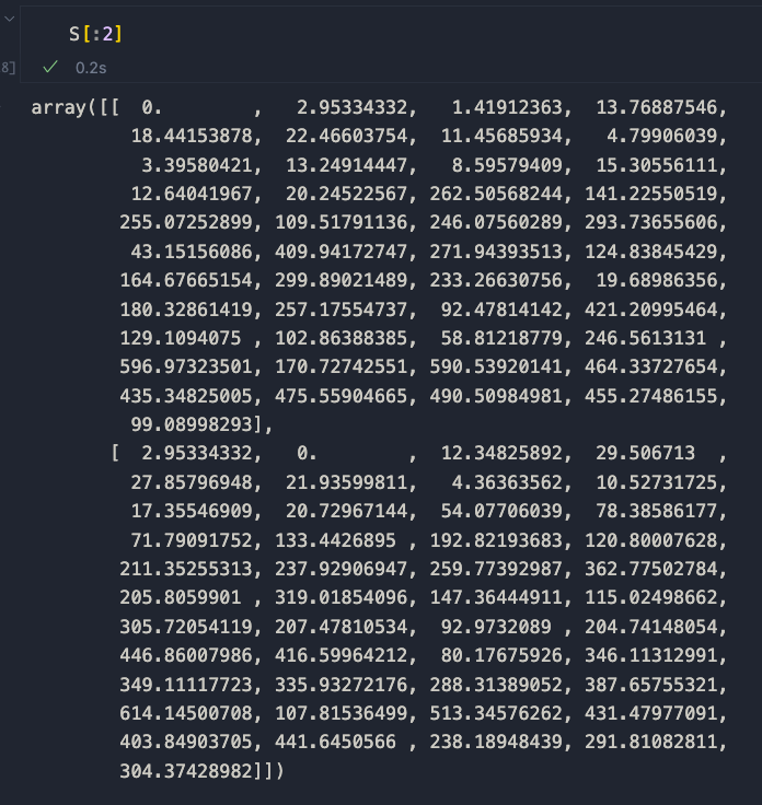
As you can see, identical series has a score of 0. Therefore, similar sequences tend to approach 0 as they become more and more similar. Let’s plot this with a heatmap.

# plot heatmap of S
fig, ax = plt.subplots(figsize=(20, 10))  
sns.heatmap(S, cmap='nipy_spectral_r', square=True, ax=ax)
plt.title("Heatmap of sequence similarities", fontsize=20, fontweight='bold')
plt.xticks(range(len(A)), range(len(A)))
plt.yticks(range(len(A)), range(len(A)))
plt.show()

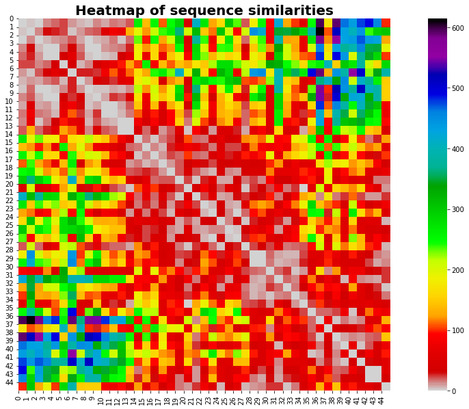
The heatmap reveals an important piece of information: the most similar sequences are found mostly at the beginning and at the end of our time series.

No idea why that’s happening — I’d be interested to hear your thoughts on this. Let’s move on.

Group similar sequences

The next step is to group similar sequences in A together. The idea here is simple: if sequences share a similarity score below a certain threshold, then group them together in a dictionary called. G. G will hold all meaningful clusters for this project.

# populate G
G = {}
THRESHOLD = 6 # arbitrary value - tweak this to get different results

for i in range(len(S)):
    G[i] = []
    for j in range(len(S)):
        if S[i, j] < THRESHOLD and i != j and (i, j) not in G and (j, i) not in G and j not in G[i]:
            G[i].append(j)

# remove any empty groups
G = {k: v for k, v in G.items() if v}

A note on the threshold: I used the value of 6 through trial and error, as it seems to produce the best results in terms of similarity grouping (check below). You may want to use other values — experiment with other values and let me know how it works for you.

Let's see how G looks like by printing a portion of the dictionary.

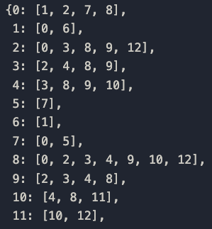
Cool…but not that cool! A dictionary doesn't really convey the information effectively. We see that some of the sequences are grouped together, but what do they look like?

Visualize the groups

And now the most exciting part of this…let’s visualize the groups!

For each key in the G dictionary, which refers to the seed sequence, let's plot the dedicated chart of all of the similar sequences.

Remember: all of the similar sequences share a low dynamic time warping value and a similar trend informed by the correlation. The parameters used to achieve this grouping are

N = 15
K = 0.70
THRESHOLD = 6

The logic seems to work just fine, as the black lines, which are the seed sequences, are surrounded by similar sequences both in terms of anatomy and direction.

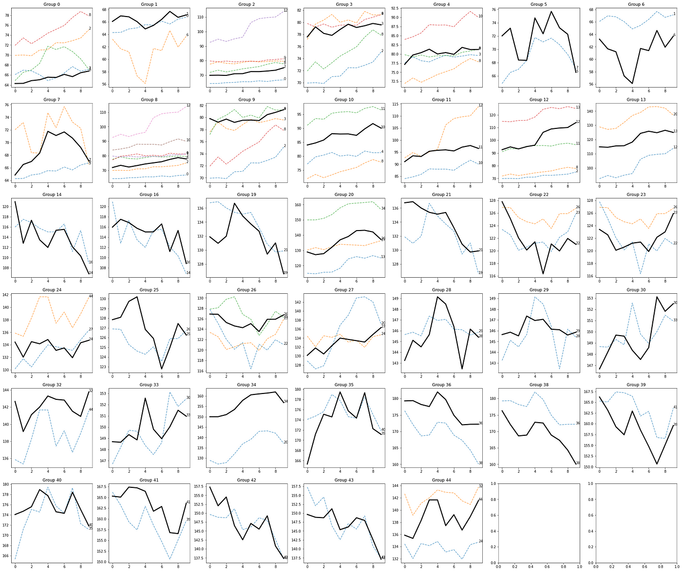
Let's check another combination of parameters.

N = 25K = 0.6THRESHOLD = 25

A new grouping of sequences based on new parameters. Image by the author.

Results can drastically change based on the input parameters. This is expected as the window size, the A/B sequence split size, and the threshold all impact the logic of the clustering algorithm.

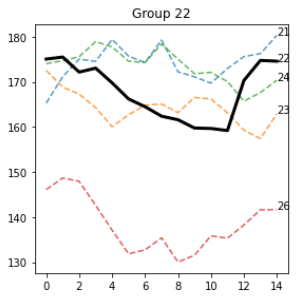
Some patterns really stand out, like this one in group 22

and group 26

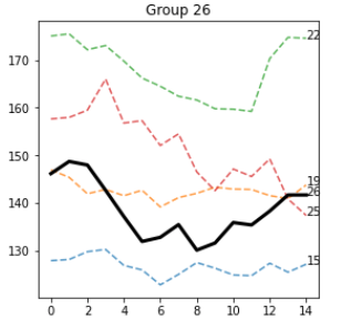
Most of the sequences around the seed sequence are indeed similar and visually share several features with the seed. I believe a more accurate methodology is required to assess these properties.

While I am sure there is a better way of computing the score, these results seem promising to me.

Compute probabilities

We approach the last section of this article. We'll now compute the probability of having an uptrend, downtrend, or stable trend for the B sequences. Recall that B always follow A — meaning that the first element of B_i follows the last element of A_i.

We'll define another helper function called classify_trend that is responsible for computing the slope and understanding the general direction of the B sequence.

def classify_trend(b, threshold=0.05):
    """
    Classify the trend of a vector
    """
    # compute slope
    slope = np.mean(np.diff(b) / np.diff(np.arange(len(b))))
    # if slope is positive, the trend is upward
    if slope + (slope * threshold) > 0:
        return 1
    # if slope is negative, the trend is downward
    elif slope - (slope * threshold) < 0:
        return -1
    # if slope is close to 0, the trend is flat
    else:
        return 0

# flatten list
flattened_G = [item for sublist in G.values() for item in sublist]
trends = [classify_trend(B[i]) for i in flattened_G]

# what is the probability of seeing a trend given the A sequence?
PROBABILITIES = {}

for k, v in G.items():
    for seq in v:
        total = len(v)
        seq_trends = [classify_trend(B[seq]) for seq in v]
        prob_up = len([t for t in seq_trends if t == 1]) / total
        prob_down = len([t for t in seq_trends if t == -1]) / total
        prob_stable = len([t for t in seq_trends if t == 0]) / total
        PROBABILITIES[k] = {'up': prob_up, 'down': prob_down, 'stable': prob_stable}

# Let's pack all in a Pandas DataFrame for an easier use
probs_df = pd.DataFrame(PROBABILITIES).T
# create a column that contains the number of elements in the group
probs_df['n_elements'] = probs_df.apply(lambda row: len(G[row.name]), axis=1)
probs_df.sort_values(by=["n_elements"], ascending=False, inplace=True)

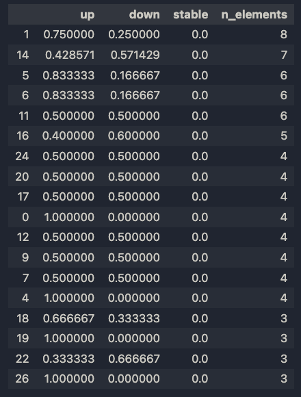
And these are the results.

Let's plot the distributions of probabilities.

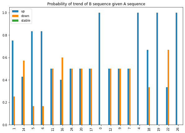
I chose to sort the items by n_elements, as the more the sequences grouped together, the more relevant the clustering. In fact, groups 1 and 14 have 8 and 7 elements, respectively, which are quite a lot of similar patterns.

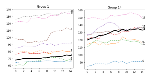
This isn't surprising, as both the A sequences are basically flat. There's definitely room for optimization here, like, for instance, removing all flat lines. But we'll look at this in the future.

In any case, 75% of the B sequences in Group 1 have an upward direction, while 57% of B sequences in Group 14 have a downward direction. Perhaps the two lines are indeed different in some aspects, or this effect is just random. Let's plot the B sequences.

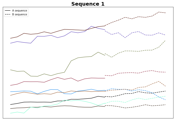
Most of these B sequences do indeed go up. There's some work to be done to ensure that this isn't just noise.

Let's check Group 14

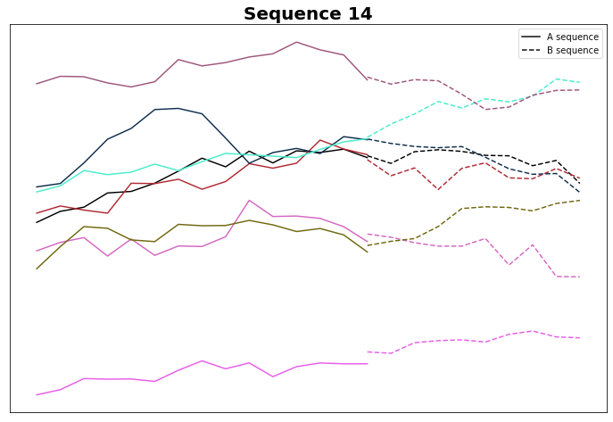
And indeed, most of them do go down. While the logic seems true to be sound, perhaps slope computation needs some refinement: perhaps we can increase the threshold from the default 0.05…but we'll look at this in the next article.

Just for pure curiosity, let's plot Group 22, which also seems interesting from the visual standpoint.

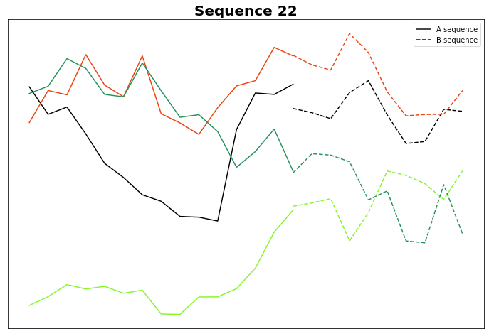
Wow. Is it just me, or do the B sequences actually look similar to one another? While this needs in-depth analysis, if this proves to be true, then A really could predict B, and this, by consequence, would explain why we see similar Bs.

Conclusion of Part 1

This has been fun. In part 1, we saw how the algorithm works and the potential it might have in predicting trends in the stock market.

Actually, if this works, it could potentially be a general approach…applicable at any time series. It is exciting! I will expand the analysis in the near future as I keep on working on the idea.

Please share your comments, doubts, and thoughts on the method. I would love to integrate feedback and contribution! 😊