Machine Learning is a discipline that is experiencing enormous development in the technological and industrial fields.

Thanks to its algorithms and modeling techniques, it is possible to build models capable of learning from past data, generalizing and making predictions on new data.

However, in some cases, models can overfit the training data and lose their ability to generalize. This phenomenon is called overfitting.

Analysts need to understand what overfitting is and why it represents one of the main obstacles in machine learning when it comes to creating a predictive model.

A general idea of overfitting is this one

When a model is too complex or fits too well with the training data, it can become very accurate for that specific data but will generalize poorly on data it has never seen before. This means that the model will be ineffective when applied to new data in real life.

Regularization techniques can be used to prevent overfitting.

The term regularization encompasses a set of techniques that tend to simplify a predictive model. In this article, we will focus on two regularization techniques, L1 and L2, explain their differences and show how to apply them in Python.

What is regularization and why is it important?

In simple terms, regularizing a model means changing its learning behavior during the training phase.

Regularization helps prevent overfitting by adding a penalty on model complexity — if a model is too complex, it will be penalized during training, which helps maintain a good balance between the model’s complexity and its ability to generalize about data he has never seen before.

To add an L1 or L2 regularization, we are going to alter the loss function of the model. This is the function that the learning algorithm tries to optimize during the training phase.

Regularization occurs by assigning a penalty that increases based on how complex the model becomes.

If we take linear regression as an example, MSE (mean squared error — read more about the evaluation metrics of a regression model here) is the typical loss function and can be expressed as

$$min_{w^{(i)}} \lbrack \frac{1}{N} \times{\sum_{i=1}^{N} (f(x_{i}) - y)^2} \rbrack$$

Where the goal of the algorithm is to minimize the difference between the prediction f(x) and the observed y.

In the equation, f(x) is the regression line, and this will have to be equal to

$$f = w^{(i)} x^{(i)} + b$$

The algorithm will therefore have to find the values of the parameters w and b from the training set by minimizing MSE.

A model is considered less complex if some parameters w are close to or equal to zero.

L1 vs L2 regularization

Now let’s see the differences between L1 and L2 regularization.

L1 regularization

L1 regularization, also known as “Lasso”, adds a penalty on the sum of the absolute values of the model weights.

This means that weights that do not contribute much to the model will be zeroed, which can lead to automatic feature selection (as weights corresponding to less important features will be zeroed).

This makes L1 particularly useful for feature selection problems and sparse models.

Taking the MSE formula above as an example, an L1 regularization would look like this

$$min_{w^{(i)}} \lbrack C \times{ (\sum_{i=1}^{N} {|w^{(i)}|})} + \frac{1}{N} \times{\sum_{i=1}^{N} (f(x_{i}) - y)^2} \rbrack$$

where C is a model hyperparameter that controls the intensity of the regularization. The higher the value of C, the more our weights will tend toward zero.

In jargon, this is would be called a sparse model, where most of the parameters have the value of zero.

The risk here is that a very high value of C will cause the model to underfit, which is the opposite of overfitting — i.e. it won’t capture the patterns in our data.

L2 regularization

On the other hand, L2 regularization, also called Ridge regularization, adds the square of the weights to the regularization term.

This means that larger weights are reduced but not zeroed, which leads to models with fewer variables than L1 regularization but with more distributed weights.

L2 regularization is especially useful when you have many highly correlated variables, as it tends to “spread” the weight across all the variables instead of focusing on just a few of them.

As before, let’s see how the initial equation changes to integrate L2

$$min_{w^{(i)}} \lbrack C \times{ (\sum_{i=1}^{N} {(w^{(i)}})^{2}} + \frac{1}{N} \times{\sum_{i=1}^{N} (f(x_{i}) - y)^2} \rbrack$$

L2 regularization can improve model stability when training data is noisy or incomplete, by reducing the impact of outliers or noise on variables.

How to apply regularization in Sklearn and Python

In this example, we will see how to apply regularization to a logistic regression model for a classification problem.

We will see how the performance changes for different values of C and compare how accurate the model is in modeling the input data.

We will use the famous breast cancer dataset from Sklearn. Let’s start by seeing how to import it, along with all the libraries.

import numpy as np
import pandas as pd
import matplotlib.pyplot as plt
from sklearn.linear_model import LogisticRegression
from sklearn.model_selection import train_test_split
from sklearn.metrics import accuracy_score

# import the dataset from sklearn
breast_cancer = load_breast_cancer()

# we create a variable "data" which contains the dataframe from the dataset
data = pd.DataFrame(data=breast_cancer['data'], columns=breast_cancer['feature_names'])
data['target'] = pd.Series(breast_cancer['target'], dtype='category')

Being a classification problem, we will use accuracy to measure the performance of the model.

Now let’s create a function to apply the comparison between L1 and L2 regularization on the dataframe.

def plot_regularization(df, reg_type='l1'):
 # we split our data into training and testing
    X = df.drop('target', axis=1)
    y = df['target']
    X_train, X_test, y_train, y_test = train_test_split(X, y, test_size=0.3, random_state=42)

 # we define the different values of C
    Cs = [0.001, 0.01, 0.1, 1, 10, 100, 1000]
    coefs = []
    test_scores = []
    train_scores = []
    for C in Cs:
     # we train the model for the different values of C
        clf = LogisticRegression(penalty=reg_type, C=C, solver='liblinear')
        clf.fit(X_train, y_train)
        # we save the performances
        coefs.append(clf.coef_.ravel())
        train_scores.append(clf.score(X_train, y_train))
        test_scores.append(clf.score(X_test, y_test))

    reg = reg_type.capitalize()

    # and create some charts
    fig, (ax1, ax2) = plt.subplots(ncols=2, figsize=(12, 4))
    ax1.plot(Cs, train_scores, 'b-o', label='Training Set')
    ax1.plot(Cs, test_scores, 'r-o', label='Test Set')
    plt.suptitle(f'{reg} regularization')
    ax1.set_xlabel('C')
    ax1.set_ylabel('Accuracy')
    ax1.set_xscale('log')
    ax1.set_title('Performance')
    ax1.legend()

    coefs = np.array(coefs)
    n_params = coefs.shape[1]
    for i in range(n_params):
        ax2.plot(Cs, coefs[:, i], label=X.columns[i])
    ax2.axhline(y=0, linestyle='--', color='black', linewidth=2)
    ax2.set_xlabel('C')
    ax2.set_ylabel('Coefficient values')
    ax2.set_xscale('log')
    ax2.set_title('Coefficients')
    plt.show()

We apply this logic by looking at the L1 regularization

plot_regularization(data, 'l1')

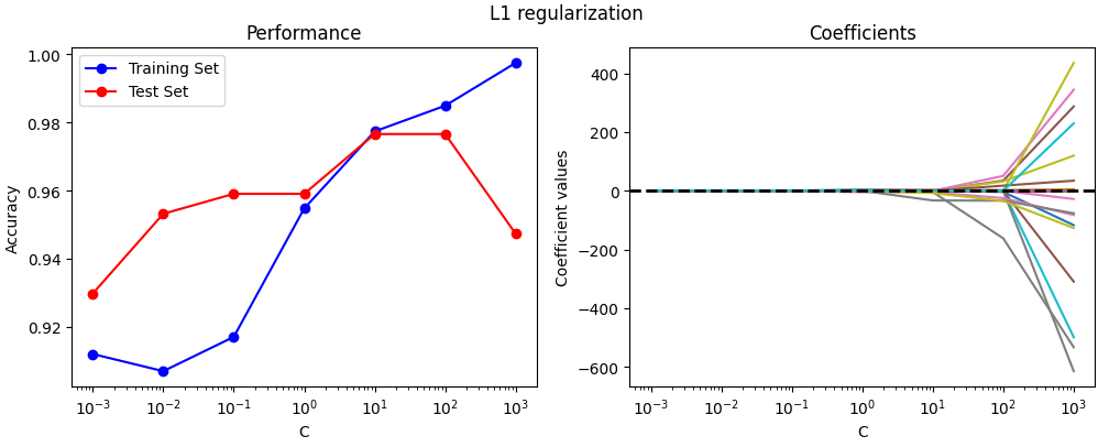
We see how the L1 regularization flattens the model coefficients close to zero for many levels of C. The coefficients with the highest values are, according to the model, the most important features for the prediction.

We also see the onset of overfitting — at C=100, the performance of the training set increases while that in the test set decreases.

We now apply the same function to evaluate the effects of L2.

plot_regularization(data, 'l2')

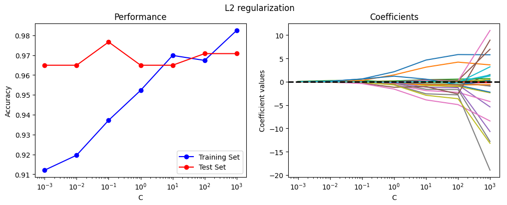
The coefficients are always above zero, thus creating a distribution of gradually increasing weights for the most relevant features. We note a very slight overfitting after the value of C=100.

Other regularization techniques

In addition to L1 and L2 regularizations, other regularization techniques can be used in machine learning models. Among these techniques, we find dropout and early stopping.

Dropout

Dropout is a technique used in neural networks to reduce overfitting. Dropout works by randomly shutting down some neurons during the training phase, forcing the neural network to find alternative ways to represent the data.

Early stopping

Early stopping is another technique used to avoid overfitting in machine learning models. This technique consists of stopping model training when the performance on the validation set starts to deteriorate. This prevents the model from overlearning the training data and not generalizing well on data not seen before.

In general, overfitting can be avoided by using a combination of regularization techniques. However, the choice of the most appropriate techniques will depend on the characteristics of the dataset and the machine learning model used.

Conclusions

In conclusion, regularization is an important machine learning technique that helps improve model performance by avoiding overfitting on training data.

L1 and L2 regularizations are the most used techniques for this purpose, but there are others too that can be useful depending on context. For example, dropout is almost always seen in the context of deep learning, that is with neural networks.

In our example, we have seen how regularization affects the performance of the logistic regression model and how the value of C affects the regularization itself. We also examined how model coefficients change as the value of C changes, and how L1 and L2 regularization affects model coefficients differently.

Thank you for taking the time to read my article! 😊

Till next time!